It was mentioned above that Green's functions should provide us with the missing link between the partial differential equations and the integral equations that "describe what is happening at a particular point in a system given information about what is happening at its boundary." There are several ways how to make this connection, some of which have already been outlined in Green's Essay.

The first way is the superposition principle.

Let us start again with the Laplace equation for the problem of a domain D with a smooth surface S.

The equation is a linear partial differential equation, so the superposition principle will work. Let us distribute N point sources at the points     on the surface S and assume that each source has intensity? () Then the following combination ( is the distance between  and x):

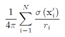
satisfies the Laplace equation everywhere except at the points.

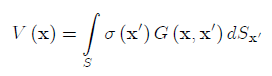
Now assume that the sources are continuously distributed along the surface S. In this case the sum in the above equation should be replaced by an integral and the solution of the Laplace equation has the following integral form:

(1)

This representation is called a single-layer potential, and the function? (x') is called a density function. The single-layer potential represents the solution of the Laplace equation at the point inside D via the data (intensities of the sources) at its boundary.

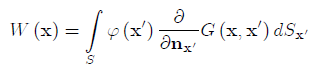
Due to the linearity of the Laplace equation, any derivative of G(x',x) over x' will also satisfy the Laplace equation everywhere except for the point x'. It is possible therefore to construct integral representations similar to that of Eq.(1) but with derivatives of G(x',x) as the integral kernels. The following representation of this kind is very important:

    (2)

Here is the normal to the surface S at the point x' and ?(x') is a density function.

Representation (2) is called a double layer potential because it can be interpreted as the limit of the sum of single layer potentials due to the sources distributed along two surfaces S and S' separated by a small distance that is let to approach to zero. The intensities of the sources continuously distributed over the surfaces are related as ?dS = -?dS'. 

Using the corresponding fundamental solutions or Green's functions, the single- and double-layer potentials can be constructed for the partial differential equations they represent (e.g. Helmholtz equation, Navier-Cauchy equations of elasticity, etc).

In his Essay, Green considered several problems with smooth surfaces. However, the excerpt from the Essay clearly demonstrates that Green fully understood the great potential of his method. Here is Green in his own words:

"The remaining part ought to be regarded principally as furnishing particular examples of the use of these general formulae; their number might with great ease have been increased, but those which are given, it is hoped, will suffice to point out to mathematicians, the mode of applying the preliminary results to any case they may wish to investigate."

And the mathematicians did just that proving the following assertion of Green:

"The applications of analysis to the physical Sciences, have the double advantage of manifesting the extraordinary 
powers of this wonderful instrument of thought, and at the same time of serving to increase them; numberless are the 
instances of the truth of this assertion."

We will get back to the mathematical developments in the Potential Theory that allowed for the relaxation of requirements on the smoothness conditions for the surfaces and density functions. Distribution Theory played an important role in these developments.

Second way. From Green to Gauss and Ostrogradsky and beyond.

In his Essay Green also formulated a very important theorem:

"Before proceeding to..., we shall in the first place, lay down a general theorem which will afterward be very useful to us. 
Let U and V be two continuous functions of the rectangular coordinates x, y, z, whose differential coefficients do not become 
infinite at any point within a solid body of any form whatever; then will..."

In modern notation this theorem can be formulated as follows:

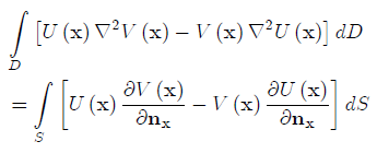
where is an external normal to the surface S. In the modern textbooks this theorem is referred to as Green's second identity. It links a surface integral of some combination of the harmonic functions and their fluxes with a volume integral containing these functions and their Laplacians.

To prove this theorem Green used what he called the method of integration by parts now known as Green's first identity which is also called Gauss' divergence theorem, named after Carl Friedrich Gauss who published it a few years after Green. Gauss' theorem is also known as  Ostrogradsky-Gauss' theorem named after Michail Ostrogradsky.

Having proved the theorem given by representation (3) Green moved further by taking one of the functions U, to be equal to the fundamental solution G(x',x), where x' is a point inside the domain D, and assuming the second function V to be a harmonic function in D. Green was fully aware that G(x',x) is a singular function, so he came up with the limiting procedure to deal with the singularity. Here is how this procedure starts:

"Then if we suppose an infinitely small sphere whose radius is a to be described around p', it is clear 
that our theorem is applicable to the whole of the body exterior to this sphere"

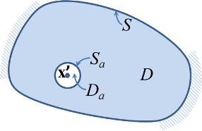
The point p' Green refers to is the point x' in our notations. So, following Green's way of thought, we take U=G(x',x)=1/(4?r) and assume that . Representation (3) can now be re-written for the volume  (figure) as follows:

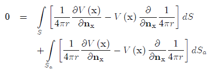(4)

where and are the volume and the surface of the sphere, respectively. The integral in the left-hand side of Eq.(3) vanishes because  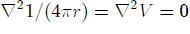in .

Using the facts that for the sphere, r = a, and, 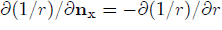, , 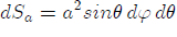where ? and ? are the angles of the spherical coordinate system with center at the point x', we can re-write the second integral in Eq.(4) as follows:

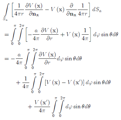   (5)

The limiting procedure in which a?0 combined with Green's assumption on the continuity of the function V results in only one non-vanishing term -V(x') in the right-hand side of Eq.(5) - so finally we get

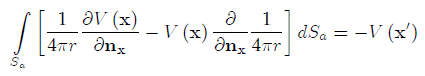
which, using Eq.(4) gives

or in a different notation

(6)

This equation is the celebrated Green's representation formula or Green's third identity.

In the case when point x' is placed outside of the domain D, the limiting process described above is not necessary, as 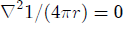  everywhere in D. So in this case

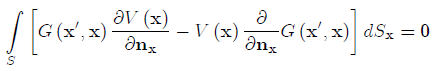(7)

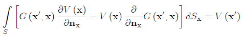
We can see that the point x is now located at the boundary S, rather than outside of it (as in Eqs.(1) and (2). The point x', on the other hand, is now located inside D. Thus, the left-hand side of Green's representation formula is a combination of a single-layer potential of Eq.(1) with the density function and a double layer potential of Eq.(2) with the density function V(x). This means that Green's formula (6) represents the value of the harmonic function at the point inside the region via the data on its surface.

Analogs of Green's identities exist in many other important applications, e.g. Betti's theorem and Somiglina's identity in elasticity, the Kirchhoff-Helmholtz reciprocal formula in acoustics, etc.

Before proceeding further we summarize the other important findings of Green's Essay, in Green's own words. Here are some excerpts from the Essay:

"Although in what precedes, we have considered the surface of one body only,
 the same arguments apply, how great soever may be their number..."

"What was before proved, for space within any closed surface, may likewise be shown to hold good,
for that exterior to a number of closed surfaces, of any forms whatever, provided we introduce the condition,
that V' shall be equal to zero at an infinite distance from these surfaces."

In addition, Green showed that the density function of the single-layer potential, Eq.(1), has a physical meaning of the following jump in fluxes

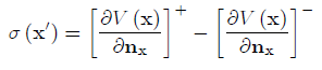 (8)

where the sign + (-) indicates that the point x' of surface S is approached (x?x') from the domain with an external (internal) normal.