Boundary integral equations | Boundary Element Method and Green's functions

From integral representations to boundary integral equations

We now have not one but several integral representations for the specific partial differential equation. However, in practically all physical problems we are looking not for the general solution of the particular PDE, but for the solution of a so-called boundary value problem This means that the solution should not only satisfy the PDE but also satisfy some boundary (and, in some cases, initial) conditions. The boundary conditions for external boundary value problems should also include the conditions at infinity.

Some boundary conditions are named after famous scientists who studied the corresponding problems, e.g. the Dirichlet boundary condition named after Johann Peter Gustav Lejeune Dirichlet; the Neumann boundary condition named after Carl Neumann; the Robin boundary condition named after Victor Gustave Robin; and the Cauchy boundary condition named after Augustin Louis Cauchy.

In his Essay Green gives the solutions to several boundary value problems. However, employing his integral representations, Green proceeds with the procedure that starts with the integral representations written for the points located either inside or outside of the boundary. The integrals are then evaluated, and only after that the point is allowed to approach the boundary, where the boundary conditions are prescribed. The unknown densities are found from those conditions. In other words, Green does not explicitly write the boundary integral equations.

Another procedure consists of allowing the field point in the integral representations of Eqs. (1), (2), (6), and (7) to approach the boundary S. The boundary conditions are then represented in terms of boundary integrals only, resulting in boundary integral equations for the unknown densities.

There were several reasons why Green used the first, "limit after the integration," procedure. One reason is given in Green's Essay:

"...we have no general theory of equations of this description, and whenever we are enabled to resolve one of them, it is because some consideration peculiar to the problem renders, in that particular case, the solution comparatively simple, and must be looked upon as the effect of chance, rather than of any regular and scientific procedure."

As we already know, Green was surprisingly well aware of the state of mathematical sciences of his time. That state is described in the review by A.T. Lonseth "Sources and applications of integral equations"

"By contrast with differential equations, which got off to a flying start with Isaac Newton's second law of motion (1687, in his Principia), integral equations arrived late; they made their first appearance, sporadically and even furtively, during the third and fourth decades of the nineteenth century. …Even the name “integral equation” was not suggested until the late 1880s, and it was adopted only in the early 1900s. In the last four or five years of the nineteenth century, Vito Volterra and Ivar Fredholm succeeded in working out fundamental linear theories of the two types which have since carried their names. Suddenly integral equations blazed forth in the mathematical heavens, a supernova heralding the analysis of the twentieth century."

The second reason for Green's approach was that the procedure of taking the limit of the potential required special care due to the singular behavior of the fundamental solutions or Green's functions. We could see that the integrals involved in Eqs. (1), (2), (6), (7) are regular, the so-called Riemann integral (named after Bernhard Riemann ), as long as the field points are located outside of S and the density functions are continuous functions. It could, in general, not be the case when the field point is taken to lie at the boundary itself. The resolution of these issues required the development of the rigorous theory of the single and double layer potentials.

The first developments were carried out by the outstanding scientists of the nineteenth and twentieth centuries Carl Friedrich Gauss, Henri Poincaré, Carl Neumann, Aleksandr Lyapunov, Vladimir Steklov. These scientists formulated what is now known as the classical potential theory (described in the book by Oliver Kellogg) that is based on the notion of Lyapunov surface and certain requirements on the smoothness of density functions.

According to this theory, the single and double layer potentials have the following limit properties.

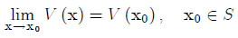
The single-layer potential of Eq.(1) is continuous function everywhere if S is a smooth surface and the density function is a continuous bounded function on S. Its limits do not depend on the way we approach the surface S; they are the same as a direct value of the integral

(9)

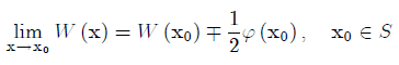
The limiting behavior of the second layer potential of Eq.(2) is more complicated. First of all, for the direct value of this potential to exist, it is not sufficient for the surface S to be smooth, S must be a Lyapunov surface. In addition, the limit values of the double layer potential do depend on the way how the surface S is approached and those values do not coincide with the direct value of the integral on S. More specifically, the links between the limit values of the double layer potentials and its direct value are

(10)

where W() is the direct value of the integral of Eq.(2) and the sign +(-) indicates that the point of surface S is approached from the domain with an external (internal) normal.

The reason for the difference in limiting behavior of the potentials is that the kernel in the double layer potential is a derivative of an already singular function. The conditions on S must therefore be strict enough to assure that W() is not a strongly singular integral.

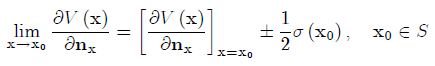
The limit properties of the potential can be used to obtain the boundary integral equations for several basic problems of Potential Theory, e.g. the Dirichlet boundary value problem and Neumann boundary value problem. However, for the latter problem, it is necessary also to know the limit values of the normal derivative dVxdnx (1).png of a single layer potential. We know from Green's Essay (see Eq.(8)) that this derivative undergoes a jump. In fact, the links between the limit values of the normal derivative of a single layer potential and its direct value are

(11)

The use of Eqs.(9)-(11) leads to the reduction of the boundary value problems to the so-called Fredholm integral equations. Those equations are used as mathematical tools to prove the existence of the solutions of various boundary value problems.

Unfortunately, here ends the analogy between the boundary value problems of potential theory and those of some other applications. Some boundary value problems, e.g. in elasticity, either can not be reduced to Fredholm's boundary integral equations (even under the strict conditions on the smoothness of the surface and the density functions) or such reductions are not beneficial.

The boundary value problems of many applications can be rather reduced to the so-called singular integral equations. It took another 60-70 years to develop solid foundations of the theory of singular integral equations. We mention just a few names of the scientists who pioneered those developments (T. Carleman, F. Noether, N.I. Muskhelishvili, V. Kupradze, S. Mikhlin, A.Calderon, A. Zygmund).

The latest developments in boundary integral equations allowed for a rigorous treatment of the problems with non-smooth boundaries and density functions and for the consideration of boundary integral equations as variational problems. We, again, mention just a few names of pioneers: V. Mazya, W. Wendland.

The later developments became possible due to the general progress in mathematical analysis that was itself stimulated by the investigations of boundary integral equations. This progress is well described in the review by A.T. Lonseth:

"Mathematicians went on energetically to generalize: David Hilbert’s geometrical way of looking at integral equations,
in “spaces” whose "points" are functions or infinite sequences of numbers, led to the active study of abstract spaces 
and their transformations: Hilbert spaces, the spaces lp and Lp of Frederic Riesz, the complete normed linear vector 
spaces of Stefan Banach in the 1920’s. Results and viewpoints of great power and generality were attained through topological 
and algebraic approaches. They reshaped the theoretical foundations of physics, especially quantum mechanics and statistical mechanics."

Thus, it became clear by the middle of the twentieth century that the boundary integral equations represent a powerful tool for solving a wide range of theoretical problems. However, their use as numerical tools was very limited. The advent of the modern digital computer changed everything.

To learn more about the ideas, history and theoretical applications of the boundary integral equations see the following references and the bibliography therein.

From integral representations to boundary integral equations

References