Ideas

The idea of the boundary element method is natural and straightforward. Here is how it was described in Jaswon’s paper that deals with two-dimensional potential problems:

"A straightforward numerical approach is to replace the equation by a system of simultaneous
 linear equations, referring to a set of nodal points spaced along the boundary L of the relevant 
domain D, these equations being assembled and solved by digital computer techniques."

The details of the numerical approach were described in the paper by G.T. Symm (http://rspa.royalsocietypublishing.org/content/275/1360/33.short), where the approach was applied to all basic equations of two-dimensional potential theory resulting from the analogs of representations (1), (2), and (6).

"To effect a numerical solution of..., we divide L into n intervals (i.e. arcs)... 
Our fundamental approximation is to assure that ?(q) remains constant within each interval..." 
so the integral equation "becomes the discrete system..."

In his seminal paper, Rizzo used the same technique to solve the integral equation of elasticity resulting from Somigliana’s identity (vector analog of Eq.(6)). The same approach was used by Crouch to solve crack problems, although the integral equations for cracks were not explicitly written: the algorithm (the Displacement Discontinuity Method) constitutes the numerical solution of the equation resulting from the elastic analog of representation (2). The density function involved in this representation has, for fracture problems, the meaning of a jump in the displacements across the crack. The numerical algorithm that constitutes the numerical solution of the equation resulting from elastic analog of the representation of Eq.(1) is described in the book by Crouch and Starfield as the Fictitious Stress Method.

Here are the main building blocks of the classical BEM algorithm:

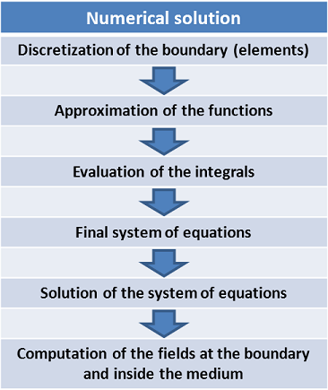
In what follows we explain how this works in the case of the so-called direct formulation based on the use of Eq.(6), which we re-write again for easy reference:

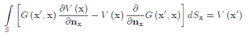
As we know the point is located inside of domain D. We now allow this point to approach boundary S. The above identity is a combination of the single- and double-layer potentials. Using the limit properties of these functions, as described by Eqs. (9) and (10), we arrive at the boundary integral equation

(12)

Equation (12) includes only the boundary values of the functions, so it is sufficient to discretize only the boundary, which means that the dimension of the problem is reduced by one.

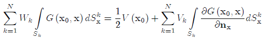
So let us assume that the boundary S is divided into N elements (e.g. triangles). We also assume for simplicity that the functions are constant within each k-th element, and equal to the values of V(x) and at some point located within the element (usually at the centroid of the element).

The discrete analog of Eq.(12) is then

(13)

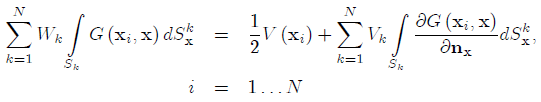
The simplest way to set up the system of equations, the collocation method, used in early papers on the BEM, consists of the sequential placement of the point at the nodes. As the result the following system of equations is obtained:

(14)

The system can be rearranged to separate known and unknown boundary values and then solved by standard numerical techniques. The fields V(x) and inside D are obtained from the discretized version of Eq.(6) and its normal derivative as follows:

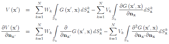(15)

We see that the latter procedure requires the evaluation of additional integrals.

As simple as it might seem the above procedure involves a number of critical issues, e.g. evaluation of singular integrals, effective methods of solution of linear algebraic systems, etc.

Much has changed since the 1960s. Over the years every aspect of the method was carefully re-examined and improved. Instead of simple constant approximations, high-order isoparametric elements became a must for accurate solutions, and algorithms that involve adaptive mesh refinement and accuracy estimations were introduced. The latter is based on the idea of a balanced combination of mesh refinement and an increase of the polynomial degree of shape functions that leads to exponential convergence of the algorithm. In the past 20 years, a considerable effort has been made on accurate treatments of integrals, especially singular and near-singular integrals.

The collocation method is not the only way to set up the linear algebraic system. This can also be done using the classical Galerkin method of weighted residuals, which assumes that the discretized integral equations are satisfied in the average sense. We can illustrate this method using Eq.(13) as an example. Integrating Eq.(13) over each element (i = 1,...,N), we get

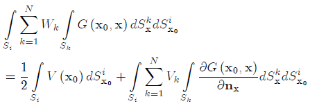(16)

The matrix of coefficients in the left-hand side of Eq.(16) is now symmetric, which is not the case in collocation method that leads to fully populated matrices. The most recent formulation, the so-called Symmetric Galerkin BEM, allows for generating a fully symmetric system of equations for all basic boundary value problems. The main idea is to properly combine the equations resulting from the representations of Eqs. (15) when x' is allowed to approach the boundary.

The invention of the Fast Multipole Method in the 1980s—labeled by the SIAM News as one of ten top algorithms of the 20th century—revolutionized the BEM. Other compression techniques (e.g. adaptive cross approximation/hierarchical matrices) allowed for fast solutions of the linear algebraic systems with millions of degrees of freedom.

In addition, new formulations were proposed such as Hybrid BEM that is based on variational principles.

The classical BEM formulations are based on the use of the superposition principle and the applicability of the specific fundamental solutions. New formulations of the BEM (e.g. Dual Reciprocity Method) are free of such limitations. In addition, several other techniques to efficiently treat the domain integrals have recently been proposed.

All recent developments in the BEM are the result of joint work by mathematicians and engineers. The National Science Foundation recognized the need for such collaboration by sponsoring two workshops in 2011 and 2012 on the Boundary Element Method: http://urbana.mie.uc.edu/yliu/NSF_BEM_Workshop/, and http://cse.umn.edu/faculty/bem/. One of the objectives of the workshops was to foster an ongoing dialog among the researchers, educators, and practicing engineers related to new areas in the field of BEM.

To learn more about the ideas of the boundary element method see the following references and the bibliography therein.

Ideas

References